BGSE Data Talks – 002 – Piotr Zwiernik

Hello and welcome to the second edition of the „Data Talks“ segment of the Data Science student blog. Today we have the honor to interview Piotr Zwiernik, who is assistant professor at Universitat Pompeu Fabra. Professor Zwiernik was recently awarded the Beatriu de Pinós grant from the Catalan Agency for Management of University and Research Grants. In the Data Science Master’s Program he teaches the maths brush-up and the convex optimization part of the first term class „Deterministic Models and Optimization“. Furthermore, he is one of the leading researchers in the field of Gaussian Graphical Models and algebraic statistics. We discuss his personal path, the fascination for algebraic statistic as well as the epistemological question of low-dimensional structures in nature.

Robert: First of all thank you very much for taking the time to talk to us. So let us start with the first question – Prof. Zwiernik, how did you get to where you are?

P. Z.: The pleasure is mine. Originally, I wanted to be a journalist and decided to study Economics. During this time I worked with Mas-Collel’s (one of BGSE’s founding fathers) classic textbook on Microeconomics and realized that I wasn’t that bad in maths. I chose to also study mathematics in Poland. Afterwards, I soon came to realize that I loved all algebraic subjects and especially algebraic geometry. Since I always wanted to combine subjects, I searched for different paths to synthesize algebra and statistics.

In 1998 the „magician“, Persi Diaconis, and Bernd Sturmfels, one of my later co-authors, published a beautiful paper, which introduced an efficient way of sampling from conditional distributions that generate specific sufficient statistics. Computational algebra provides a set of moves that allows us to connect the sampling space. Afterwards, one just has to run a standard MCMC algorithm such as Metropolis-Hastings. This beauty led to me focusing on the geometry of graphical models during my PhD studies in statistics at the University of Warwick.

At UC Berkely, during one of my many post-docs I was actually able to meet Professor Diaconis in person and had opportunity to participate in Michael Jordan’s working group. In Jordan’s group we read many papers, which covered completely different topics. But still we were able to find deep connections. This helped me realize, what people were really interested in. Nowadays, I tackle problems, which lie in the intersection of algebraic geometry and high-dimensional statistics.

Robert: How did your Economics background affect the path that you took and how does it influence your way of thinking?

P. Z.: First of all Economics introduced me to the field of Econometrics and statistics in general. Doing research in Econometrics also showed me the difference between theory and working with real data. We should never forget: Working with data is hard. Really hard.

One of my personal heroes is Terry Speed, who went through a very interesting transformation. He started of by studying pure geometry. Afterwards he got interested in statistics and cumulants. Only in the end he decided to work with real data and contributed research in the field of Bioinformatics. I can imagine traveling a similar path.

Robert: Can you tell us more about your post-doc time in the US? How did it compare to your experiences in Europe and did you feel pressured to succeed in the academic world?

P. Z.: In my mind the time of being a post-doc is the time of exploration. During mine I realized that everything is connected with each other. Hence, no time and effort is ever completely wasted. There is always something you can take away from studying a topic. It is extremely hard to do research if you constantly want to prove yourself. During the years I observed many colleagues, who burned themselves exactly because of this. The take-away message: Free exploration of the world is key and you should not stress yourself too much.

The academic world in the US is not very homogenous. Berkeley for example has a strong focus on optimization and Computer Science. Chicago and Seattle, on the other hand, specialize more on structural and algebraic problems – on how things really work.

Nandan: How do you define „making progress in understanding“?

P. Z.: This is a tough question and I will try to answer it with a recent example: Total positive distributions. One example of these can be found in so-called one-factor models, which are commonly used in psychometrics. Specific abilities (e.g. logical reasoning and spatial understanding) are assumed to be conditionally independent given a latent variable (e.g. intelligence). Usually these abilities are also positively correlated and this phenomenon seems to be characteristic for many natural systems. Sometimes it is only approximate (like Gaussianity), but still it is omnipresent. For example two undergraduate students of mine studied high-dimensional portfolio selection and were able to show that the covariance matrix of stocks exhibits strong traits of total positivity. This is only one example. Every few years it feels like I reach a new milestone of understanding. 

Robert: Can you also give us a philosophical and intuitive understanding of your fascination for algebraic statistics?

P. Z.: Algebra is all about finding patterns in nature and different subfields of mathematics. The world is full of symmetrical relationships, which we try to detect. Thereby algebra simplifies and unifies the language, researchers use. Personally, I am interested in models that exhibit this symmetry property.

Gaussian Graphical Models are just one instance of this class of models. Another beautiful property of them is that there are many different ways, in which we can express them:

1. They can be formulated from a  statistical physics point of view. The joint distribution can be written as the product of factor functions.
2. Furthermore, we can also express them with the help of classical graph theory. Nodes represent variables. Missing edges represent conditional independence relationships. Each graph represents a specific factorization of the joint distribution.
3. Finally, they can also be studied as parametrized distributions such as in the exponential family setting. This allows us to make use of ideas from the theory of convexity, combinatorics and decomposable graphs.

There are endless connections, which brings me back to one of my previous points: Everything is related. Making connections and exploiting links is the way how we make progress.

Robert: In the previous year and in our convex optimization class we spoke a lot about penalized likelihood models and the underlying assumption of sparsity in nature. Do you think this assumption holds?

P. Z.: Not in the sense that the causal relationship between some variables has to be 0. But I believe in the hypothesis that nature’s underlying factors lie on a lower-dimensional manifold. Nature tends to fall in love with low-dimensional structures, which are not generic but very special. One such example is the Fibonacci Sequence. Low-dimensionality can have many different faces (e.g. sparsity or low-rank matrix factorizations). But often times people just assume the form, which is computationally tractable.

Nandan and Robert: You are also the organizer of the Statistics and Operations Research seminar at UPF. Can you tell us more about it, your future plans and the importance of a flourishing research community?

P. Z.: First of all, we have a very limited budget. This means that we are very much focused on inviting European researchers. Everyone knows Pompeu Fabra for its outstanding research in Economics. But not many people know us for our work in statistics or mathematics. Our overall goal is to change this. And our strategy is twofold: First, we invite strong senior researchers, who are great speakers. The speakers are exposed to the research group and the group can benefit from external stimuli. Second, we also invite young researchers, who work in fields close to our own. This gives them the opportunity to collaborate with us in the future and also helps us to increase our reach.

In the past we have had the fortune to host prominent guests such as Caroline Uhler (MIT), Wilfrid Kendall (Warwick) and Bin Yu (Berkeley). So we are slowly but surely progressing. For the future we want to invite more researchers. Also, the newly assembled Data Science Center is going to generate new sources of funding. We are hoping to be able to invite at least one very good speaker from the US per year.

Having a flourishing local community is extremely important! Our small group works extremely well together. For example, Eulalia Nualart, who is a theoretical probabilist, has written multiple papers with Christian Brownlees, who mainly researches in time series analysis. Mihalis Markakis and Gabor Lugosi started working on bandit problems together and in general there is a friendly and open atmosphere at UPF. All of us are doing very distinct things, so there are many opportunities to learn from each other.   

Nandan and Robert: Lets wrap this up by asking you for your ultimate advice for all PhD students and aspiring Data Scientists? What do you wish you could have known earlier?

P. Z.: Don’t think about research as a way to prove yourself, but as an exploration process of the world. David Blackwell, one of the brightest statisticians ever, once said: „Basically, I’m not interested in doing research and I have never been. […] I’m interested in understanding, which is quite a different thing.“

Nandan and Robert: Thank you very much Professor Zwiernik! 

References

Diaconis, Persi, and Bernd Sturmfels. “Algebraic algorithms for sampling from conditional distributions.” The Annals of statistics 26.1 (1998): 363-397. 

Dudoit, Sandrine, ed. Selected Works of Terry Speed. Springer Science & Business Media, 2012.

Prediction as a Game

Introduction

In this article we provide a general understanding of sequential prediction, with a particular attention to adversarial models. The aim is to provide theoretical foundations to the problem and discuss real life applications.

As concrete examples consider the following three real-life situations:

1. Every Sunday you can choose either to go on trip to Costa Brava or to study in the library. To go on trip you need to buy tickets the day before. You want to be sure that you will enjoy a sunny day. Basing your decision on a single weather forecast might not be a good idea and you consider multiple forecasts. How to take the “best” possible action in the presence of experts’ advise is an issue that we address in this article.

2. After getting too much rain at the beach and studying on sunny days, you gave up on going on trip but to compensate you decide to go out for a dinner every Saturday. Your objective now is to pick the best possible restaurant based on your preferences – or most likely on your girlfriend’s preference – but you know very few restaurants in Barcelona. We will address this issue by studying a strategy for the so called multi-armed bandit problem.

3. Every month some friends are visiting you. Once they arrive you always have to recommend a restaurant where they can go on themselves – while you are studying in the library. Once they go to the restaurant you ask for a feedback, but you always receive partial or even no feedbacks from your lazy friends. This problem can be modeled as a partial monitoring multi-armed bandit problem that we describe in the last session.

For completeness of the article we provided a proof to our statements whenever this would not make the discussion too heavy. The reader might skip the proof if not interested.

Sequential prediction: General Set Up

Before entering into the discussion we provide a general set up. Considers being the outcome space. The forecaster chooses an action where is the decision space and she has a loss at time , . To be concrete, in Example 1 the loss might be 1 if you either you went to the beach when raining or you were studying with sunny weather, 0 otherwise.

In an oblivious game the environment chooses the outcome regardless of the strategy of the opponent. We define the cumulative loss of the forecaster. Without loss of generality we can impose that .

The regret at time for choosing action instead of action is defined as . A natural objective function is the average maximum regret faced by the forecaster, defined as: .

Considering again Example 1, if you went to the beach on a rainy day but all did the same because all experts told you that it was going to be sunny your regret would be simply 0.

Forecasting strategies that guarantee that the average regret goes to zero almost surely for all possible strategies of the environment are defined Hannan consistent.

Prediction with experts advice

We start our discussion first considering the context of regret minimization for prediction with experts advice [3] under a convex loss function. With an abuse of notation we consider the decision space being of each expert .

Prediction protocol with convex loss function
For each round

1. the environment chooses the next outcome without reveling it;
2. each expert reveals its prediction to the forecaster;
3. the forecaster chooses ;
4. the environment reveals ;
5. the forecaster suffers the loss and each expert suffers a loss

Consider the following strategy:

with
, , .

Then this strategy is consistent at a rate proportional to .

This results show that by assigning exponential weights to each forecaster you will end up with a strategy consistent at optimal rate.

Notice that this result strongly relies on the assumption of convexity on the loss function. In the next session we relax this assumption and show that you can get similar results.

Proof.

Considers log() = log() – log() = . Then a lower bound can be defined as

Notice then that , with . Given that the loss is bounded between 0,1, by Hoeffding inequality:

By Jensen’s inequality

Therefore we get . Rearrenging things we get

By the first order conditions on the upper bound we choose and by substituting the term we get:

Sharper bounds can be obtained by imposing some structure on the behavior of the loss function.

New Prediction Protocol

For each round

1. the environment chooses the next outcome without reveling it;
2. each expert reveals its prediction to the forecaster;
3. the forecaster chooses a probability vector over the set of M actions and draws an action 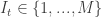with

4. the environment reveals ;
5. the forecaster suffers the loss and each expert suffers a loss

In this case the average regret is bounded by with probability at least .

Again the strategy is consistent at optimal rate. The importance of this result relies on the fact that now we have a consistent strategy for deciding which weather forecasts believe to for any possible loss we have in mind! In the next session we go through a technical proof that the reader might prefer to skip if not interested in the details of the theorem.

Proof.

To prove the result we first make use of the following lemma:

Lemma 1. Let being a random variable such that , where is the filtration at time . Then by Hoeffding-Azuma inequality

Proof of Lemma 1. By the Chernoff bound for some . By using the law of iterated expectations and by Hoeffding inequality

The argument can be repeated times and get . Using this result and minimizing over gives the result shown in the previous expression.

We can now move to the actual proof. Define where is the filtration at time . Furthermore, notice that is a martingale and has expectation . Using Hoeffding-Azuma
w.p. , therefore the loss are concentrated around expectation. Notice now that is convex (linear in this case) in the first variable. Therefore by the previous result

By adding and subtracting :

which concludes the proof.

Multi-Armed Bandit Problem
We now move to the problem of choosing the best restaurant without knowing many restaurants and without the help of TripAdvisor!

Consider the following prediction protocol:

Prediction Protocol: Multi-Armed Bandit Problem

For each round

1. the environment chooses the next outcome without reveling it;
2. the forecaster chooses a probability vector over the set of M actions and draws an action ;
3. the forecaster suffers the loss ;
4. only is reveled to the forecaster, the loss for all other actions remain unknown.

The objective function of the forecaster remains the regret. Clearly the situation is much more challenging, provided that there is not common knowledge of the loss incurred at every time by each expert. We define the following unbiased estimator:

where is the probability of choosing action at time and is the indicator variable equal to 1 if is true, 0 otherwise. Notice that

A forecasting strategy in Multi-Armed Bandit Problem

We define the gain and the estimated unbiased gain. Notice that is at most 1, a property used for a martingale-type bound. Choose . Initialize .

For each round

1. Select an action according to the probability distribution ;
2. calculate the estimated gain:
3. update the weights ;
4. update the probabilities with exponential weights.

Note that by introducing a parameter we give up the unbiasedness of the estimate to guarantee that the estimated cumulative gains are, with
large probability, not much smaller than the actual cumulative gains.
Under conditions of theorem 6.10 [2] the regret is again. Therefore even without having no clue about what the loss would have been by going to new restaurants the strategy is consistent at optimal rate!

Discussion

We want to stress that the main ingredients for an optimal rate of convergency in probability are contained in the exploration-exploitation trade off. In fact notice that

then the first term multiplying by contains information regarding the losses of the actions taken in the past. The second term instead let the forecaster have non-zero probabilities for exploring new actions. In practice, the strategy give you a guide for how many times you should explore going to new restaurants and how many times you should go to good restaurants where you have already been.

Partial Monitoring Multi-Armed Bandit Problem

As a further motivating example of a partial monitoring regret minimization problem consider the following dynamic pricing model.

A vendor sell a product to customers one by one. She can select a different price for each customer but no barganing is allowed and no further information can be exchanged between the buyer and the seller. Assume that the willingness to pay of each buyer is , the actual price offered to the seller is and the loss incurred by the seller at time is

with . The seller can only observe whether the customer buys or not the product and has no clue about the empirical distribution of . A natural question is whether it exists a randomized strategy for the seller such that the average regret is Hannan consistent.

In a more general setting we define the following prediction protocol:

Prediction Protocol: Partial Monitoring Multi-Armed Bandit Problem

For each round

1. the environment chooses the next outcome without reveling it;
2. the forecaster chooses a probability vector over the set of M actions and draws an action ;
3. the forecaster suffers the loss ;
4. only a feedback is reveled to the forecaster.

The losses of the forecaster can be summurized in the loss matrix . With no loss of generality . At every iteration the forecaster chooses an action , suffers a loss but she only observes a feedback parametrized by a given feedback function that assigns to each action/outcome pair an element of a finite set of signals. The values are collected in the feedback matrix . Notice that the forecaster at time has access only to the information . In [1] the following strategy was shown to be Hannan consistent at a sub-optimal rate .

Assume that , that is , considering and having the same rank. Define and as an unbiased estimator of the loss:

with being the probability of having chosen action at time and . Initialize . For each round

1. Let and ;
2. choose an action from the set of actions at random according to the distribution defined by

3. let for all

In [1] the authors shown that under some mild conditions the strategy has a performance bound with a magnitude proportional to , that is with a convergency rate . Interestingly in the scenario of a simple multi-armed bandit problem, whenever , the theorem leads to a bound of order , much slower compared to the result obtained in the previous section. Finding the class of problems for which this bound can be improved remains in fact a challenging research question

Discussion

We have just shown that it exists a consistent strategy even without having full information on the loss that you incurred, as in the case of the third example in the introductory session, but at a slower rate.

RandNLA for LS: A Brief Introduction – Part II

In the previous article we took a first look at the pioneering work of Michael Mahoney and Petros Drineas in Randomized Numerical Linear Algebra. Our ultimate goal was to speed up the computation of the ordinary least-squares solution vector, , from time to at least time. We reviewed two simple and fairly “slow” but powerful algorithms which simplified linear systems of equations with a large number of constraints (the classical setting of tall data). The main idea was to preprocess the input matrix in such a way that we obtained a “representative” sketch in a lower dimensional space (). The term “representative” could be defined in two different ways and always with respect to the ultimate goal: a good approximation to the least squares (LS) solution. First, a good representation in a lower dimensional space could be interpreted as a subspace embedding that maintains pairwise distance up to an -degree (via Johnson-Lindenstrauss transforms). This idea was the fundament of a random projection algorithm. Second, “representative” could be defined in terms of “leverage” on the LS fit. A natural measure was the so-called statistical leverage score, which could be extracted from the diagonal elements of the hat matrix or from the euclidean row norm of the orthonormal basis for computed from the QR decomposition or SVD.

The main difference between the two methods was that the projection approach was data-agnostic. This meant that we did not have to compute any statistics in the first place. Sampling on the other hand involved some serious preprocessing in the form of establishing an importance sampling distribution. Both methods have advantages and disadvantages: Computing the exact leverage score (random sampling) was associated with a full singular value decomposition. Computing the SVD is usually (disregarding sparse variants) already as expensive as solving the complete LS problem in the first place. Furthermore, it is unclear whether or not leverage is a “robust” measure of being a representative sample from the underlying data-generating process. Eliminating one high-leverage observation might dramatically affect the complete sampling distribution. On the other hand, computing the ordinary Johnson-Lindenstrauss transform in the random projection variant using a dense matrix would take at least time (matrix-matrix multiplication). Since usually , we would not obtain an improvement.

In todays article we are going to introduce the Fast Johnson Lindenstrauss Transform (FJLT). This result is going to be the fundament of two very important concepts which speed up the computation of an -approximation to the LS objective function and the target vector: First, the FJLT can be used to quickly project the original data matrix into an -dimensional subspace, in which the leverage scores are uniformized. In this way we are able to sample rows uniformly at random. Secondly, it is also going to allow us to approximate the actual leverage scores in a fast way. Both concepts rely on Fast Fourier (or Hadamard-based) transforms. Ultimately, this is going to speed up computational complexity from to .

The following text is structured in the following way: First, I introduce the concept of a Fast Johnson Lindenstrauss subspace embedding. Afterwards, I will outline a fast random sampling algorithm for LS. In the end, we will analyze complexity and discuss further research questions as well as possible extensions/improvements. Again, the main reference is Mahoney (2016).

1. The Fast Johnson Lindenstrauss Transform

Remember that the goal of all our efforts is to approximate the solution of a system of linear equations by a vector and to do this in a reasonably fast way (faster than ). The main ingredient for this is going to be the fast brother of the regular Johnson Lindenstrauss transform: The fast subspace Johnson Lindenstrauss transform. Mahoney (68, 2016) defines it in the following way:

Definition 1 (Fast Johnson Lindenstrauss Transform – FJLT) Given an and an orthogonal matrix viewed as d vectors in . A FJLT projects vectors fro such that the orthogonality of U is preserved, and it does it quickly. I.e., is an -FJLT if

• Orthogonality preservation:
• Fast: we can compute in time.

The first condition requires us to maintain the orthogonality of the orthonormal basis U even after processing it with . So how can we define such a matrix? Ailon et al (2006) proposed the following Hadamard-based construction, which relies on fast Fourier/Hadamard preprocessing of the input matrix:

• – Sparse JL matrix/Uniform sampling matrix (Achlioptas (2003), Frankl et al (1988)), where 
  
• – DFT or normalized Hadamard transform matrix: Structured so that Fast Fourier methods can be applied to compute them quickly. Setting it is defined for all that are a power of two in a recursive fashion :
• – Takes values with probability each: Preprocesses bad cases by randomization.

The matrix product fulfills two very important tasks (Drineas et al, 3449, 2012): First, it essentially flattens spiky vectors (“spreads out its energy” – Drineas et al (3449, 2012)). Mathematically speaking, this means that we can bound the sup-norm of all transformed vectors by a quantity that is inversely proportional to . This ultimately uniformizes the leverage scores (leverage scores will equal ). If is large enough, this smoothing in combination with the sampling matrix allows us to construct an FJLT with high probability. Furthermore, computing the vectors of the FJLT transformed matrix can be done in , as desired. Hence, can be viewed as a subsampled randomized Hadamard transform (Drineas et al, 3449, 2012) or as a FJLT with high probability.

In this way, we obtain two potential algorithms for solving the above LS problem (Mahoney, 71, 2016):

• (i) Random Projection Approach II: Uniformize leverage scores and use sparse projection matrix (or sample uniformly)
• (ii) Random Sampling Approach: Use FJLT to compute approximate leverage scores and sample accordingly

In the next section we will focus on the second approach. There is no particular reason, except that we are going to be able to introduce a new idea in approximating the quantity that allows us to approximate our objective by random sampling.

2. Doing things faster

Before we are able to outline the full random sampling algorithm we need to find a fast way to compute the leverage scores. We saw that the exact computation was done by computing the SVD. But this did not speed things up. We can fasten this process by applying the previous trick a second time: We will not calculate the exact leverage slowly but calculate an approximation (with -slack) in a fast way. Drineas et al (2012) first proposed the following algorithm to approximate the leverage scores:

Drineas et al (3451, 2012) – FJLT approximation for leverage scores

Input:  with SVD  and an -level
Output: Approximate leverage scores,  
-----------------------------------------------------------------------------------
Let  be an -FJLT for  with . 

Compute  and its SVD/QR where . 

View the rows of  as n vectors in . Let  be an -JLT for  vectors, with . 

Return , an -approximation of .

It relies on first applying a FJLT to . Afterwards one has to compute the SVD of the transformed matrix, before applying another regular JLT to . The complexity of the algorithm can be decomposed in the following way:

• takes since is an -FJLT
• SVD of takes
• takes since is an -JLT
• Premultiplying by X takes (plain matrix-matrix multiplication)
• Overall:

By choosing the parameters appropriately (, , constant, , ), it follows that the algorithm has complexity .

Using these fast leverage score approximations, we can construct an importance sampling distribution and apply the following algorithmic leveraging algorithm first introduced by Drineas et al (2011):

Drineas et al (2011) – “Fast” Random Sampling Algorithm for LS

Input: LS problem with ,  and an -level of approximation 
Output: Approximate LS solution,  
---------------------------------------------------------------------------------
Compute the importance sampling distribution , where  and  are the orthogonal matrices from either the SVD or the QR. 

Randomly sample  rows of  and . Rescale them by  and form .  

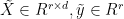Solve  using any of the above mentioned algorithms. 

Return , an -approximation of .

So what makes this algorithm work in practice? Given that is large enough, the two crucial structural conditions on (see below) are going to be fulfilled by the subsampled randomized Hadamard transform:

Both of them are needed to obtain a proof for the following quality-of-approximation result such as in Drineas et al (2011). They essentially allow us to find explicit bounds on , which in turn can be used to bound the randomized residual sum of squares (see Drineas et al (2011) for complete proof). This again bounds the possible deviation the randomized estimator can take from the least-squares solution:

Theorem 1 (Least Squares Quality of Approximation) The returned vector of algorithms 1 and 3 is such that with probability at least 0.8

where is the condition number of and denotes the fraction of the norm of that lies in the column space of :

In order to asses the statistical properties of this estimator, I construct Monte Carlo experiments which are displayed in the figure below. The left figures plot the ratio of the euclidean norm approximation error of the random sampling estimator (compared with the true data generating vector) and the right-hand-side of the quality-of-approximation result for the solution certificate. In 1000 simulation runs I draw samples of independently normal distributed data (). Afterwards I multiply with a five dimensional vector and add some noise to obtain . For each one of the 1000 samples I compute one random sampling estimator and take the euclidean norm of the difference. The resulting figure plots the histogram and a corresponding kernel estimator. The right figures, on the other hand, plots a comparison of a simple Cholesky decomposition based least squares estimator, . The estimators in the first row randomly sample according to the leverage scores. We can directly see that the above theorem holds. More than 0.8 of the probability mass lies below 1. Hence, in at least 80 percent of the cases holds. Furthermore, it becomes apparent that the random sampling estimator does a way better job at approximating the estimator instead of the true data-generating vector . Intuitively, this makes a lot of sense: One of LS well-known weaknesses is its sensitivity to outliers. Outliers often times have large leverage scores which translate into a higher weight in the sampling procedure, which underlies the randomized estimator. Hence, the weakness of LS is going to be forwarded to the randomized estimator. We can conclude, that the random sampling estimator does a very good job at what it is intended to do: Provide an approximation to the least-squares estimator.

In order to obtain a more robust estimator one may use influence scores instead of leverage scores. Influence scores are supposed to be a more insensitive measure and are defined in the following way:

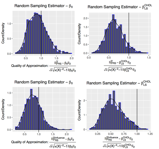
While the leverage scores completely ignored any information in the response vector , influence scores incorporate this information. We easily compute the influence scores by appending to the design matrix and computing the diagonal elements of the hat matrix of this new matrix in . This seems only natural since we are constructing sketches of not only but also . The second row of the figure displays the empirical distribution of the quality of approximation result for the estimator based on the influence scores. The estimator clearly performs better in both situations!

3. Open Research Questions and a Bunch of Potential Applications

As we have seen, RandNLA is a powerful framework that allows us to speed up solutions to fundamental linear algebra problems. It can basically be applied to any ultra-high-dimensional matrix-matrix multiplication and linear systems of equation problem, that you can imagine. Therefore, RandNLA has a huge potential. My master thesis, for example, is going to deal with an application to Generalized Linear Models (GLMs) and the family of exponentially linked models. Furthermore, one could think of applications in deep learning. Many architectures already make use of randomization in form of stochastic gradient descent and dropout. The main reason for this is, that it helps avoiding to get stuck in local optima. Maybe one could also obtain the similar results by working with random sketches and exact gradients. If you are interested and want to chat about it, feel free to contact me! Again, the code can be found on my GitHub.

References

Achlioptas, Dimitris. “Database-friendly random projections: Johnson-Lindenstrauss with binary coins.” Journal of computer and System Sciences 66.4 (2003): 671-687.

Ailon, Nir, and Bernard Chazelle. “Approximate nearest neighbors and the fast Johnson-Lindenstrauss transform.” Proceedings of the thirty-eighth annual ACM symposium on Theory of computing. ACM, 2006.

Drineas, Petros, et al. “Fast approximation of matrix coherence and statistical leverage.” Journal of Machine Learning Research 13.Dec (2012): 3475-3506.

Drineas, Petros, et al. “Faster least squares approximation.” Numerische Mathematik 117.2 (2011): 219-249.

Frankl, Peter, and Hiroshi Maehara. “The Johnson-Lindenstrauss lemma and the sphericity of some graphs.” Journal of Combinatorial Theory, Series B 44.3 (1988): 355-362.

Mahoney, Michael W. “Lecture Notes on Randomized Linear Algebra.” arXiv preprint arXiv:1608.04481 (2016).

Statistical Racism

I got into a brief discussion about policing and profiling, in the context of the United States, with someone the other day. He immediately asked me:

“You don’t actually believe the police should equally stop old white ladies as often as they do young black men, do you? That would be completely inefficient.”

I stared at him.

I believe the moral issues with profiling are understood by most, whether they are bothered by them or not. There’s a lot of discussion about structural inequality, which is clearly a complex topic, but I thought that most people would be fairly clear on the basic concept: treat people unequally, people will become unequal (or even more unequal).

This guy was supposed to be an econometrician, but it doesn’t take one to know that more young black men are arrested than old white ladies. There are a lot of ways in which policing can affect crime, but we don’t even need the real-life nuances and complexities of this issue to make clear the problems with profiling. We can pretend policing has no affect other than catching true criminals, and we can assume that young black men truly are more likely to commit a crime. Even with these generous assumptions, there is an even more basic statistical problem with profiling:

We don’t actually know who is committing crimes. The only thing we can know is how many are caught.

Let’s assume we go out, on day one of the world, and stop people uniformly. After day one, we get the following distribution of caught criminals:

Let the x-axis be any quality that can be policed: income, geography, skin-color, etc. Clearly, in our population, there is some group that is more likely to commit crime than the others. This group is in the center of the x-axis. We have a choice on day two: how to we police this population? Should we stop everybody uniformly, again, or should we focus on those in the center, those more likely to commit a crime?

Let’s assume the police continue their uniform policing. In other words, every single day, regardless of yesterdays distribution of criminals, the police stop people at completely at random, and haul in whoever happens to be a criminal. We will simulate this process 50 times to see what happens after 50 days:

If you sample uniformly from a distribution, you get back that same distribution.

On day 50, however, things change in our little world, because on day 50, our ambitious new police chief hires in a crack consultant to develop a stats-driven policing strategy! The crack consultant takes a look at their graph of criminality. We can use this past data, she claims, to predict crimes and catch even more criminals. She points to the mode of the distribution, and tells them that if they sample from the mode, they will always have a higher probability of catching a criminal than if they sample from anywhere else.

This feels a bit too extreme for our until-now-relatively-moderate police department, so they settle on a compromise. It’s less efficient, but a little more fair, they feel: they will stop people with probability equal to the probability that that person, according to the data, will commit a crime. They still police everyone, but now they’re being more efficient!

Simulating the effect of efficient policing, now taking into account the x-axis of the individual and using their probability to commit crime as the probability of stopping them, we see how the numbers start to shift even after a single day of the new policy:

If you sample un-uniformly from a distribution, you don’t get the same distribution back.

I just finished an excellent book by Cathy O’Neil, called Weapons of Math Destruction. I would consider it an important book. Cathy explores, through dozens of contemporary, solid examples, the negative societal implications of naive implementation of statistical learning algorithms. In it, she makes concrete this exact scenario we are exploring here. She explores the software being developed and sold to police departments that predicts future crime based on past data.

In the real-life algorithms being implemented by police departments, as in our toy simulation, the data used to find criminals is not the data on crimes, but the data on crimes caught.

On day 52, our aspiring department uses, quite naturally, the data from day 51, which offers the most accurate predictions as to who will predict crime. The police are most definitely catching more criminals, but they are also biasing their statistics, and when those are the same statistics being used to catch the next batch of criminals, you have structural inequality.

This is what structural inequality looks like after 100 days of efficient policing:

Our police department has slowly, unwittingly, implemented the exact “efficient” strategy that the consultant originally proposed: sample from the mode, you will catch the most criminals. The police department is definitely working efficiently, if we narrow our definition of productivity to number of criminals caught, but they’ve created a whole new problem.

I’ll leave it to others to discuss the implications of the above distributions, the implications that structural inequality has for our society. But I hope this simulation has at least proved the statistical reality of the situation.

For those curious, here’s the code used for the simulations and graphs:

	using Distributions
	using Gadfly
	using StatsBase
	using KernelDensity
	using DataFrames
	function generate_population(n::Int, d::Sampleable)
	# Create population, with criminals distributed according to
	# the provided distribution (d)
	x = rand(n) * 20 – 10
	y = [pdf(d, i) > rand() ? 1 : 0 for i in x]
	collect(zip(x,y))
	end
	function catcher(population, estimate, unif::Bool)
	# If we are sampling uniformly, pick 1/10 of the population at random,
	# otherwise, use the previous estimated density function to sample.
	sampler = !unif ? x -> pdf(estimate, x) > rand() : x -> 1/10 > rand()
	# Stop people according to our sampling strategy. If we find
	# a 1, that indicates a criminal, and we catch them.
	stopped = [(x,y) for (x,y) in population if sampler(x)]
	caught = [x for (x,y) in stopped if y == 1]
	# Restimate a probability density based on those we caught
	estimate = InterpKDE(kde(caught))
	caught, estimate
	end
	function simulate(n::Int, K::Int, unif::Bool, d::Sampleable = Normal())
	# Generate our initial population
	pop = generate_population(n, d)
	# Run the catcher K times
	caught, _ = reduce((t, _) -> catcher(pop, t[2], unif), ([], d), 1:K)
	# Return the original criminals as well, to compare
	true_criminals = [x for (x,y) in pop if y == 1]
	caught, true_criminals
	end
	function create_df(caught, badguys)
	[DataFrame(x = caught, Distribution = "Caught");
	DataFrame(x = badguys, Distribution = "True Criminals")]
	end
	function resample(n::Int, K::Int, unif::Bool, d::Sampleable, geom, coords)
	caught, badguys = simulate(n, K, unif, d)
	df = create_df(caught, badguys)
	plot(df, x = "x", color="Distribution", geom, coords)
	end
	to_svg(plots) = [draw(SVG(n, 7inch, 5inch), p) for (n, p) in plots]
	d = Cauchy(0, 10)
	geom = Geom.density(bandwidth = 3)
	coords = Coord.cartesian(xmin=–10, xmax=10)
	to_svg([("day-one.svg", plot(x = simulate(1000000, 1, true, d)[2], geom, coords)),
	("uniformly-50.svg", resample(100000, 50, true, d, geom, coords)),
	("efficient-one.svg", resample(100000, 1, false, d, geom, coords)),
	("efficient-100.svg", resample(100000, 100, false, d, geom, coords))])

view raw

racists.jl

hosted with ❤ by GitHub

BGSE Data Talks – 001 – Ioannis Kosmidis

In this series we interview professors and contributors to our fields of passion: computational statistics, data science and machine learning. The first interviewee is Dr. Ioannis Kosmidis. He is Senior Lecturer at the University College London and during our first term he taught a workshop on GLMs and statistical learning in the n>>p setting. Furthermore, his research interests also focus on data-analytic applications for sport sciences and health.

Nandan: First of all thank you very much for taking the time to talk to us. We are very eager to learn more from you, so lets get started with our first question: Which papers have fundamentally changed the way you think?

Kosmidis: There many papers that have deeply affected me, but let me give you my top 3:

The first one is a paper by Bradley Efron from 1975. Statisticians have known that procedures and models that are linear (e.g. canonically-linked exponential family models) have nice properties in learning and inference problems.  In his paper Efron provided a framework that describes of how much one can deviate from these linear cases before these good properties start deteriorating. It’s a beautiful paper, which concentrates elements from 70 years worth of statistical thinking. Furthermore, it is accompanied by an amazing discussion, including topics on the construction of confidence intervals, second-order efficiency and unbiased estimators. All of these concepts are put under the same umbrella, and quantified by one key quantity: the statistical curvature. This is one of the papers that helped me a lot in my own research and made me think hard on the models I use and the impact they have on what I want to achieve with an analysis.

The second paper is well known to graduate students in Data Science: Leo Breiman’s paper about the two cultures in statistics and machine learning – inference and prediction. In that paper, Breiman has a  pro-prediction attitude, arguing that the relevant problems are prediction-based. One of my favorite parts in that paper is actually Cox’s commentary. Cox tries to balance Breiman’s enthusiasm for prediction in a very elegant way. He argues that optimal prediction, as a target is often dangerous; in many settings in statistics you are faced with the following problem. Data can only be collected under certain conditions but predictions are only useful under a different set of conditions. For example, think of modeling the spread of a new dangerous virus.  Of course you wouldn’t have past data on its behavior. So without any idea of the dynamics you are trying to model and by using a black box prediction algorithm, you might get strong predictive results, which are actually useless for the question at hand. One of the things that  a statistician ought to be good at is to recover data-generating mechanisms, test scientific hypotheses, and develop the means to do so.

And finally, there is a wonderful report by Donoho, which is called ’50 Years of Data Science’. Starting with the fundamental work by John Tukey, Donoho outlines the history of our craft. He asks fundamental questions about what defines a “Data Scientist” and how Data Science should be taught. He comes up with a list of courses, which a Data Science program should include. For example, I fully agree with his proposal to include a course on “Legal, Policy, and Ethical Considerations for Data Scientists”. Furthermore, a course, which takes an in-depth look at the connection between causality and experimental design should find a home in every Data Science program. Clever experimental design is key for good inference.

It is really important to be clear about which question you are trying to answer and to stay open whenever a new data analytics setting comes in. You can’t answer everything with a neural network. In some cases it is much better to have a model with only few parameters, which actually explains something. In this way subject matter experts are able to improve their work.  This is much harder with complex black boxes.

Robert: Successful companies such as Google DeepMind, SpaceX and Alphabet Inc. are largely focused on optimizing certain prediction tasks by building complex models (Deep Reinforcement Learning, etc.). Do you think that this hype could pose a potential danger for the state of inference?

Kosmidis: No, not at all. Such developments are hugely important and very inspirational. In order to understand these systems we need complex models. But this is not all. These extremely non-parametric models often give you a baseline, something to try to outperform with a model that encodes common sense and scientific knowledge, and can be used for inference on relevant hypotheses.

Robert: What do you think about p-value manipulation and the fact that so far (almost) only significant effects are being published in economics, social sciences and psychology? Does scientific evolution really apply to those fields?

Kosmidis: In 2011 Jonathan Schooler proposed in a Nature paper to introduce a repository of negative or non-important results. Whenever you get a non-important result, there are two things that might have happened: There is actually no effect or you have used the wrong methods to try to discover an effect. If we had a repository of all those analysis, one could try and re-attempt them.

A move towards  raising awareness of the issues you are referring to is the ASA’s statement on p-values from 2016. The statement outlines 6 things p-values are not and is signed by well-known scientists.

Nandan: Coming to one of your key research areas – Data analytics for health and fitness. How do you imagine our data driven health system evolve in the next 10 to 20 years?

Kosmidis: I imagine that there is going to be a huge revolution in data analytic solutions for health and fitness. All of us carry many devices that can now communicate in a very efficient way with each other. They collect data on a regular schedule and can update us on the potential actions we should take to improve, for example, our fitness. In a sense, the algorithms will be able to map the data that we generate to our idea of the future, an putting together inference and prediction, you as a user will be able to intervene to yourself, online.

Nandan: Jumping to another topic: What are the most valuable, annoying or essential attributes of Phd students that you have supervised or hope to supervise in the past or future? And is there any final advice you can give to young and aspiring Data Science students?

Kosmidis: I believe that the most important quality for a PhD student is curiosity.

My advice: Keep an open mind!

Robert and Nandan: That wraps it up. Again, thank you very much for your time and thoughts. It was a pleasure to learn from you.

REFERENCES

Breiman, Leo. “Statistical modeling: The two cultures (with comments and a rejoinder by the author).” Statistical Science 16.3 (2001): 199-231.

Donoho, David. “50 years of Data Science.” Princeton NJ, Tukey Centennial Workshop. 2015.

Efron, Bradley. “Defining the curvature of a statistical problem (with applications to second order efficiency).” The Annals of Statistics (1975): 1189-1242.

Schooler, Jonathan. “Unpublished results hide the decline effect.” Nature – 470.7335 (2011): 437.

Wasserstein, Ronald L., and Nicole A. Lazar. “The ASA’s statement on p-values: context, process, and purpose.” The American Statistician (2016).

RandNLA for LS: A Brief Introduction – Part I

Dimensionality reduction is a topic that has governed our (the 2017 BGSE Data Science cohort) last three months. At the heart of topics such as penalized likelihood estimation (Lasso, Ridge, Elastic Net, etc.), principal component analysis and best subset selection lies the fundamental trade-off between complexity, generalizability and computational feasibility.

David Rossell taught us that even if we have found a methodology to compare across models, there is still the problem of enumerating all models to be compared. At this point the bias-variance trade-off turns into a question of computational power. Evaluating every single model using Bayes Factors or other performance measures just becomes way to expensive if the number of potential predictors exceeds 30 ( models). Instead of going the brute force way, one usually makes use of computational heuristics, which are clearly associated with short-comings. But what if we could sketch each model performance measure up to a certain degree of certainty?

Randomized Numerical Linear Algebra (RandNLA) is a fairly new and hot research field, which intends to speed up fundamental linear algebra operations by making use of either random sampling or random projections. The ultimate aim is to compress dimensionality in a sensible manner while obtaining an ()-approximation of the objective. The top names in this field are Drineas, Kannan and Mahoney (2006 a,b,c). All of them have done pioneering work in the field of randomized algorithms for large matrices. Their work covers a whole branch of computational approximations such as randomized versions of matrix-matrix multiplication, least squares (LS), fast leverage score approximations and sparse matrix completion. The following two-part-series is mainly based on lecture notes of Mahoney (2016) and intends to introduce the audience to an alternative randomized perspective on solving the standard LS problem. Therefore, this article is going to review two simple (and fairly “slow”) but powerful ideas which simplify linear systems of equations with a large number of constraints (the classical setting of tall data). The next article is going to improve upon these two algorithms by widening the computational bottlenecks. Thereby we are able to speed up computational complexity from to . So lets get started!

The Translation of the LS Problem

The standard LS problem can be summarized in the following optimized objective function (RSS)

where , and . After “doing the math” (multiplying out, taking the gradient, yada yada) LS boils down to solving the following normal equations

Usually, this system is solved using Cholesky, QR decomposition or the SVD. The complexity of all methods is (different constant factors – depending on how well-conditioned is).

Randomized algorithms intend to work on the tall -side of things (although it is also easily possible to switch sides). Instead of crunching the full matrix and n-dimensional response vector , we want to do something smart: Construct a sketch of and , and , which drastically reduces the amount of rows to . Let’s write the transformed objective function as where denotes some transformation matrix. Afterwards, we solve this reduced system and obtain the vector . There are two objectives which we intend to achieve:

Clearly, the second objective is more relaxed than the first. The solution space that fulfills the second objective is a subset of the solution space for the more strict first condition. Usually, it only kicks in if the solution certificate is hard to achieve in the first place. The natural question that pops up is: What are reasonable structural requirements to an approximation scheme?

Mahoney (2016, 57) states the following two: Let X = denote the singular value decomposition of . Furthermore, let denote the residual vector, resulting from the fact that not all of can be “reached” by (Note ).

The first structural condition states that we require a lower bound on the singular values of . This basically means that we want to be an approximate isometry/rotation after reducing the dimensionality to r  (Mahoney (2016, 57)) . Hence, the transform is not allowed to influence the original problem and therefore the fit too much.

Standard LS minimizes the RSS by orthogonally projecting y onto the column space of X. The orthogonal projection is described by a linear combination defined by . The second structural condition therefore requires that this orthogonality approximately “survives” the transformation. Hence, has to be approximately orthogonal to . All of the following algorithms are going to fulfill these conditions (for proofs see Mahoney (2016)). One can already tell that the number of dimensions on which we reduce, has to be related with the quality of our approximation. All proofs essentially work out the -r-trade-off by making use of matrix concentration inequalities.

A First Slow Random Sampling Algorithm

can be viewed in two different ways: Either as a sampling matrix or as a projection matrix. Let us first consider the former case: This clearly has to be a non-data-agnostic way of constructing (we have to do computations with X to obtain some sampling reference). Each row of contains one non-zero entry, which represents a rescaled sampled row (Note: We sample with replacement). Intuitively we want to sample observations that highly influence the original LS fit more often. A natural measure of influence of each data point on the in-sample fit of itself is the statistical leverage. It tells us how much a specific data point pulls the linear model fit towards itself. A data point with leverage 1 “occupies” one complete parameter/degree of freedom. Hence, we are interested in computing the diagonal elements of the hat matrix and sample according to exactly these leverage score probabilities. It can be shown that and hence we have a first potential randomized algorithm:

Mahoney (2016, 65) – “Slow” Random Sampling Algorithm for LS

Input: LS problem with ,  and an -level of approximation 
Output: Approximate LS solution,  
--------------------------------------------------------------------------
Compute the importance sampling distribution , 
where  and  are the orthogonal matrices from either the SVD or the QR. 

Randomly sample  rows of  and . Rescale them by  and form . 

Solve  using any of the above mentioned methods. 

Return , an -approximation of .

As described above, we basically construct a sampling distribution by computing the exact leverage scores. The problem with this algorithm is that computing the SVD of is already almost as expensive as solving the full problem in the first place. Hence, we need a fast way to compute an approximate leverage score. Before addressing this issue in the following article, let us take a look at a different point of view: dimensionality reduction through random projections.

A First Slow Random Projection Algorithm

Random projections are based on one key result (and many different versions), the Johnson-Lindenstrauss Lemma and the resulting transformation.

Lemma – Soft Gaussian-version of Johnson-Lindenstrauss Lemma (Mahoney (2016, 45))

Given n points , each of which is in , let  be such that 
 and let  be points in  defined as .  
Then if , for some , then with probability at least 0.5, 
all point-wise distances are preserved,  we have 

Pause for thought – this is an amazing result! Instead of having to precompute any metric before being able to do anything, there is an easy way to obtain a lower dimensional representation of our original input, that preserves the original length and point-wise distances. The proving argument is based on a combination of the Chernoff bounds and Boole’s inequality and can again be found in Mahoney (2016, 46 et seq.).

Definition – Johnson-Lindenstrauss Transform (Mahoney (2016, 68))

Given an  and  points , where , an -JLT (-
Johnson-Lindenstrauss Transform), denoted  is a projection of the points 
into  such that

 

The Johnson-Lindenstrauss Transform maps the n-dimensional row vectors into a r-dimensional subspace, while preserving their length and their point-wise distances up to an -proportion!

Most of the constructions of are either based on Gaussian random samples or on binary coin tosses (Achlioptas, 2003). In terms of computational efficiency, binary coin tosses are a lot faster! This is due to the fact that simulating Gaussian samples (e.g. Box-Mueller algorithm for transformation of uniform samples) is usually a lot harder than just tossing a fair coin. The general version of this algorithm looks like this:

Mahoney (2016, 65) – “Slow” Random Projection Algorithm for LS

Input: LS problem with ,  and an -level of approximation 
Output: Approximate LS solution,  
--------------------------------------------------------------------------
Construct a random projection matrix  of Gaussians or binary  coin flips. 

Randomly project onto  rows of  and form . 

Solve  using any of the above mentioned methods.

Return , an -approximation of .

Sadly, also this algorithm has computational downsides associated to the computation of the matrix-matrix product of and which already has a complexity of .

Computational Bottlenecks and an Outlook

The presented randomized algorithms provide an )-approximation to the LS objective function value and an -approximation to the solution vector. But the ultimate goal of all our effort is to speed up computation time. Sadly, both of the proposed algorithms do not improve on the complexity of standard LS algorithms.

In the random sampling algorithm computing the SVD to obtain exact leverage scores is almost as expensive as solving the whole problem LS in the first place. Computing the matrix-matrix product of in the projection scenario already has the complexity of which is usually larger than . Widening these bottlenecks is going to be part of the next article (Hint: In both cases we are going to have to make use of Fast Fourier or Fast Johnson-Lindenstrauss-Transforms (Ailon and Chazelle, 2006).

The process is going to heavily rely on smart data-preprocessing and the use of fast projection methods. This will enable us to either construct fast approximate leverage scores and to sample according to this importance sampling distribution (Fast Random Sampling). Or to approximately uniformize the leverage scores by projection, which will allow us to sample uniformly at random (Fast Random Projection). If you are interested in an R implementation of the algorithms in this blog post please check out my github repo (here).

References

Achlioptas, Dimitris. “Database-friendly random projections: Johnson-Lindenstrauss with binary coins.” Journal of computer and System Sciences 66.4 (2003): 671-687.

Ailon, Nir, and Bernard Chazelle. “Approximate nearest neighbors and the fast Johnson-Lindenstrauss transform.” Proceedings of the thirty-eighth annual ACM symposium on Theory of computing. ACM, 2006.

Drineas, Petros, Ravi Kannan, and Michael W. Mahoney. “Fast Monte Carlo algorithms for matrices I: Approximating matrix multiplication.” SIAM Journal on Computing 36.1 (2006 a): 132-157.

Drineas, Petros, Ravi Kannan, and Michael W. Mahoney. “Fast Monte Carlo algorithms for matrices II: Computing a low-rank approximation to a matrix.” SIAM Journal on Computing 36.1 (2006 b): 158-183.

Drineas, Petros, Ravi Kannan, and Michael W. Mahoney. “Fast Monte Carlo algorithms for matrices III: Computing a compressed approximate matrix decomposition.” SIAM Journal on Computing 36.1 (2006): 184-206.

Mahoney, Michael W. “Lecture Notes on Randomized Linear Algebra.” arXiv preprint arXiv:1608.04481 (2016).

About the Author

I (Robert Lange) graduated last year from the University of Cologne with a BSc in Economics. Reading Milton Friedman’s “Essays in positive economics” and a passion for computational statistics led me to pursue a more empirically driven path. I quickly realized that there is only one Master’s  program in this field that is suited to fulfill the needs of the 21st century: Data Science at the Barcelona GSE. Ultimately, I want to combine data-analytic knowledge with problems that change the way  we pursue of lives (e.g. Bionformatics and Neuroscience). If you are interested in me, check out my homepage.

Covariance matrix estimation, a challenging research topic

Covariance matrix estimation represents a challenging topic for many research fields. Sample covariance matrix might perform poorly in many circumstances, especially when the number of variables is approximately equal or greater then the number of observations. Moreover, when the precision matrix is the object of interest the sample covariance matrix might not be positive definite and more robust estimators must be used. With this article I will try to give a brief (and non-comprehensive) overview of some of the topics in this research field. In particular, I will describe Stenian shrinkage, covariance matrix selection through penalized likelihood and graphical lasso implementing the description with some potential extensions of these methodologies.

As shown by Wolf and Ledoit, 2004, the sample covariance matrix can be written as where and , where P is the number of variables and N the number of observations. Because the rank is bounded by the minimum of the rank of the two matrices, whenever P is greater then N the matrix is not full rank.

When instead but their ratio is close to one, the problem is very likely to be ill-conditioned and different estimators are needed especially to compute the precision matrix. Intuitively, “S becomes unstable in the sense that small perturbations in measurements can lead to disproportionately large fluctuations in its entries” (Chi and Lange, 2014).

How to find the weighting parameter is a crucial issue. Wolf et al., 2004, minimized the expected quadratic distance between the true and the estimated covariance matrix based on the Froebenius norm in the context of portfolio risk optimization. Therefore, the objective function that they proposed is , where is replaced with its sample estimation. The researchers used asymptotic properties to justify their choice. On the other hand, as shown by Zhou et al, 2010, the rate of convergence under the Froebenius norm depends on the both the number of observation and the dimension of the problem. Therefore, we felt that in high dimensional settings a complementary approach in the context of portfolio risk minimization might be by estimating the weighting constant using cross validation. In a project developed by 4 current Data Science students, described in an upcoming article of this blog, they proposed the following methodology for portfolio risk minimization: every four months, they selected a sequence of alpha from 0 to 1, they computed the corresponding covariance matrix and the best capital allocation according to the given matrix. They kept the portfolio for the subsequent two months and then they computed the variance of the returns under the given portfolio during the two-months period. The process was repeated for daily returns of 800 random companies for a sample of 8000 companies from 2010 to 2016. They finally selected the lowest alpha leading to the lowest average out of sample variance. The best alpha was around 1/2, while for values lower then 0.44 the matrix was singular as expected. This methodology might be effective when the target loss function depends on some other model specification. On the other hand, this method has many computational limitations and it might be infeasible in many circumstances. In this context both missing values and the choice of the subsample might have had affected the result in an unknown way.

A different approach for covariance estimation consists in solving a penalized regression problem in order to estimate the covariance matrix (Pourahmadi et al, 2006). The idea comes from a well-know link between the entries of the precision matrix and a regression problem. To show this, each variable can be described as: , where is gaussian noise centered on zero. By assuming for the moment that , we can identify a projection matrix containing the coefficients such that and where is a vector of residuals, is the identity matrix and X is a vector of observed values. Taking the variance of the residuals we know that: where D is a diagonal matrix containing the variance of the residuals. It can be shown that we can express the off diagonal elements of H as a function of the precision matrix K: . This properties have been exploited in many settings. Pourahmadi et al. proposed a parametrization of the concentration matrix using the generalized Cholesky decomposition for time serie analysis. For time series, the coefficient is the auto-regressive coefficient, where each serie is regressed on the previous observations. The generalized Cholesky decomposes the matrix into LDL, where L is a triangular matrix with ones elements on the diagonal and D is a diagonal matrix. The matrix L can be interpreted as the matrix , containing the negative coefficients on the off-diagonal elements of the upper triangle, ones on the diagonal – each observations is not regressed on itself- and zero in the remaining entries. The matrix D instead is the positive diagonal matrix containing the residuals variance. By imposing and therefore by shrinking the regression coefficients, the entire concentration matrix can be shrunken towards a more robust estimator. The objective function proposed is the log-likelihood of the data depending on , the residual variance for each observation at time t, and the regression coefficients. Interestingly, the best tuning parameter can be known using the generalized cross validation formula which provides a closed form approximation to leave-one-out cross validation for any linear regressors (The elements of Statistical Learning, ch.7, Tibshirani et al.).

We feel that the two approaches, apparently very different each other, might be linked, although further investigation is necessary in this field. The LDL decomposition provides a map between the precision matrix and the hat matrix, considered the necessary component to find the tuning parameter by using a closed form approximation to cross validation. On the other hand the MLE approach with shrinkage might be computational costly in terms of number of parameters to be estimated. The Stenian shrinkage instead is cheap in terms of the computation of the entries of the two matrices, but the main challenge consists in finding the best weighting parameter. Therefore, if there exist a map between the of the Stenian shrinkage and the for a shrinkage of the regression coefficients, then the two approaches might overlap and some computational gains could be achieved. One possible way could be to compute a set of matrices corresponding to a sequence of the weighting parameters , under the Stenian model and then compare the performance of each matrix using generalized cross validation by exploiting the generalized Cholesky on the given Stenian covariance matrix. On the other hand this has not been proposed in any paper and more investigation is necessary to assess the correctness of this approach.

Many other methodologies for shrinkage of the covariance matrix exists. A further alternative approach is by estimating the covariance by maximizing the log-likelihood expressed as where S is the sample covariance matrix and . According to Tibshirani et al., 2008, we can express the problem by imposing an additional term representing a penalty on the sum of the L1 norms of the entries. The imposition of the penalty ensure sparsity whenever the tuning parameter is large enough.
There are many extensions to this problem. The general idea is to minimize the likelihood function by imposing some given constraints. Many alternative approximations have been proposed in recent years – e.g. penalize the nuclear norm of the matrix – and many other approaches have been studied.

References

Cai, T. Tony, Cun-Hui Zhang, and Harrison H. Zhou. “Optimal rates of convergence for covariance matrix estimation.” The Annals of Statistics 38.4 (2010): 2118-2144.

Chi, Eric C., and Kenneth Lange. “Stable estimation of a covariance matrix guided by nuclear norm penalties.” Computational statistics & data analysis 80 (2014): 117-128.

Friedman, Jerome, Trevor Hastie, and Robert Tibshirani. “Sparse inverse covariance estimation with the graphical lasso.” Biostatistics 9.3 (2008): 432-441.

Hastie, Trevor, Robert Tibshirani, and Martin Wainwright. Statistical learning with sparsity: the lasso and generalizations. CRC Press, 2015.

Huang, Jianhua Z., et al. “Covariance matrix selection and estimation via penalised normal likelihood.” Biometrika 93.1 (2006): 85-98.

Ledoit, Olivier, and Michael Wolf. “A well-conditioned estimator for large-dimensional covariance matrices.” Journal of multivariate analysis 88.2 (2004): 365-411.

About the author(Davide Viviano)

I graduated in Economics at Luiss University with an experience of studies at UBC, Vancouver and a very brief experience of research in Econometrics. My interest in both theoretical and applied research in many fields of statistics was the main reason to enroll in the Data Science Program at BGSE.

Competition Report: Monster Legends Datathon

Just a few days after officially starting our classes for the 1st term in the master program, we received an email about a gaming data hackathon being organized by SocialPoint – a big name in mobile gaming. The company is spread across 7 floors of a 10-storey building in the heart of Barcelona with amazing views of the city. Having just finished the brush-ups, we were not quite aware of the kind of data challenges that lay ahead in such competitions but it was surely going to be a learning experience so we went ahead and registered a team.

We arrived at the venue on the morning of 15 Oct to learn about the challenge at hand. We were provided with gameplay data from the company’s most successful game Monster Legends. For our readers with some time at their disposal (not quite the case with most of us doing the master), you should try this game but I shall warn you it can be addictive! The basic aim of the game is to collect the strongest monsters and build up your team of monsters to win the maximum battles against other players. And this brings me to the problem we had to solve: Given the list of monsters currently owned by a player, predict the monster they don’t already have and are most likely to choose next.

We were given:

• A training dataset of 70,000 players and all the monsters they owned.
• A test dataset of 30,000 players with one random monster removed from their list of monsters – This removed item was to be predicted
• Basic information about each of the 100,000 players (country, sex, platform, days_played, payer_dummy etc)
• Features of each monster available in the game
• A baseline Item Based Collaborative Filtering (IBCF) model in R which gave an accuracy of 15.5%

There were 2 tracks on which each team would be judged:

1. Objective evaluation of the precision of the predictions which was accessible through a live leaderboard – it evaluated the submissions on 20% of the solutions to avoid overfitting.
2. Subjective evaluation of a Business Insights presentation which was supposed to be delivered the next morning with suggestions to SocialPoint about how to possibly increase revenue from the game, given our analysis on the provided data.

There were cash prizes for both tracks – 1st and 2nd prize of €750 and €500 for the accuracy track and a unique prize of €500 for the business insights track.

We would be presenting our results to – Horacio Martos (CEO, SocialPoint), Sharon Biggar (Head of Analytics, SocialPoint), Manuel Bruscas (Director of Analytics, eDreams) and our program co-director Christian Fons-Rosen.

With all this information at our disposal – the countdown timer for 24 hours started and we put on our thinking caps to brainstorm. We began with visualizing as much data as possible to get a general sense of the data provided. Apparently our brains were waiting for some calorie intake as only after the lunch (which was a fancy courtesy of the organizers), we came up with a basic idea of modeling the game as chronological event and predicting the monster for a player based on the player’s current level.

2 of us set on to implement this approach while the other 2 continued tweaking the baseline model in hopes of achieving a better precision. However, we failed to cross the 15% mark after several submissions coupled with hours of stackoverflowing and reading about various techniques.

Much to our disappointment, our chronological approach also didn’t give very optimistic results and DeepYellow (our team) was still lingering around 17% by the time we left the venue on Saturday evening. Some of us stayed up all night trying to implement different ideas – clustering players on features other than level and other techniques like user-based filtering. I believe the competitiveness of the event with regular submissions by all teams even at 3AM and the idea of trying new models kept us going.

After all our efforts, we were still at 19% at the end of 24 hours and clearly not the winning the team – the winners managed to achieve 37% accuracy. Given our unsuccessful attempts at analyzing the data – we were not really motivated about the presentation and we gave a very basic one which was not really very insightful. However, we learned a lot from the presentations of the other teams.

At the end of the event, we were given a tour of the offices and we got back to our lecture slides albeit not with cash prizes but with ideas on practically facing a data problem and hopefully some acquired knowledge. Hackathons are always a fun way of squeezing out the creative side in you in a limited amount of time coupled with the bonus of meeting many like-minded new people.

Our team consisted of Akhil Lohia, Nandan Rao, Robert Lange and Roman Kopso (an exchange student at UPC who was included in our team to assure all teams had 4 members).

About the author (Akhil Lohia):

I graduated with a bachelor’s degree in Economics from the Indian Institute of Technology Kanpur in June 2015. I have been involved in economics research projects in the capacity of a research assistant. My deep fascination towards technology and the ever increasing involvement of data to augment and provide more useful services to users in their context led my decision in choosing the Data Science program at BGSE in a smart city like Barcelona.

Finding an optimal group allocation

The Task

During our first week of class, the BGSE Data Science class of 2017 was asked to form groups of 3 (and one group of 4) for the upcoming group projects of the first term. The question on-hand was how and on what basis to form these groups.

After some discussions, we decided to go with the following approach: Each of the 25 students provides a ranking of fellow students from 1 (most preferred) to 24 (least), considering the people’s’ previous academic background, interests, career aspirations, etc. From this input we would then compute the group allocation that is collectively most favorable, i.e. which minimizes the sum over the group member links, weighted by their ranking.

Finding the optimum solution to this problem turned out to be non-trivial. In the following I shall discuss a possible solution to that problem.

Representation as Graph
First, note that the problem on hand can be formulated as a complete, undirected graph where each student represents a vertex and the edge’s weight between 2 vertices A and B forms the sum of the rank of student A for student B and vice versa. The aggregated rank matrix therefore becomes the adjacency matrix of that graph.

The goal now is to form complete subgraphs of size 3 (and one subgraph with 4 vertices) such that the total weights of used edges gives the minimum.

Brute-Force
A graph with 25 vertices allows for over  different combinations of group allocations:

A brute-force approach – i.e. computing all possible combinations and then picking the combination with the minimum total edge weight – can therefore be deemed infeasible.

Literature Review

The next step was to review the literature for similar algorithmic problems and associated efficient solutions.
The stable matching (or marriage) problem considers finding a stable matching between two equally sized sets of elements given an ordering of preferences for each element. It differs from our problem in that each vertex is associated with one of two groups and it only allows for pair-wise matching. Furthermore, the solution to the problem is stable (i.e. no two individuals have an incentive to re-match) but not necessarily optimal from all individuals’ points of view.
In the similar stable roommate problem all elements (roommates) belong to a single pool, however, the problem is still restricted to pair-matching and the efficient algorithm by Irving (1985) does not generalize to larger groups.

Proposed Algorithm
With no ready-to-use algorithm on hand, we were forced to design a new group-matching algorithm.
The proposed algorithm starts from any valid solution and then iteratively improves the solution by swapping unstable pairs of students from different groups. The produced solution is therefore guaranteed to be stable for pairs of individuals but not necessarily for 3 or more individuals trading “under-the-table”. From that follows that the algorithm is likely to find a “good” solution but not necessarily an optimal solution.

The pseudo-code of the algorithm  is given below:

INPUT: adjacency matrix, group_sizes
OUTPUT: group allocation
--------------------------------------------------------------------------
form groups of given group sizes
initial solution: randomly assign vertices to initial groups
--------------------------------------------------------------------------
WHILE solution has changed
     FOREACH pair of vertices (i,j)
        cur_cost <- sum(edge weights of i)
                              + sum(edge weights of j)
        alt_cost <- sum(edge weights of i if in group(j))  
                              + sum(edge weights of j if in group(i))
        IF alt_cost < cur_cost
              swap i and j

Complexity

The algorithm compares   pairs of students in each WHILE loop. In the worst case, the algorithm could start from the worst possible solution and in each WHILE loop iteration only move to the next-best solution, thus leading to brute-force-like performance.

Tests with an implemented version of the algorithm (in R), however, showed that for graphs of size 25, the algorithm converges after an average of 20 swaps and no more than 3 WHILE loop iterations. Thus, the algorithm is believed to be efficient in the average case.

Further tests with different initializations for the same rank matrix confirmed that the algorithm only converges to a local minimum in the solution space. It is believed that the algorithm produces a good solution when run several times with different initializations and then choosing the solution with lowest total cost, however, by no means it can be guaranteed to have found the global optimum solution.

Final Note
The described group allocation process based on rankings turned out to be not self-enforcing and therefore was not actually used in the end.

References
Irving, Robert W. (1985), “An efficient algorithm for the “stable roommates” problem”, Journal of Algorithms, 6 (4): 577–595, doi:10.1016/0196-6774(85)90033-1

About The Author (Hans-Peter Höllwirth):
I have several years of working experience in the software industry as programmer, analyst, and project manager, and graduated from the University of Edinburgh with a bachelor degree in Computer Science and Management Science in 2016. My interests in machine learning, computing, and finance led me in my decision to join the BGSE Data Science program.

 

 

 

 

return(„Hola mundo“)

Hello and welcome to the 2016/2017 edition of the Data Science Blog!

I know it is already a little late for the first entry but we have big plans for the future: hackathon reports, technical essays, interviews and personal diary entries are only a few of those. Our general aim is to inform you about all the wonderful details of our experience at the Barcelona Graduate School of Economics and the specifics of the Data Science program.

If there are any topics or questions you are particularly interested in, please let Nandan (nandan.rao@barcelonagse.eu) or me (robert.lange@barcelonagse.eu) know.

Next week Hans-Peter Höllwirth is going to write about one of the first practical problems we encountered during our Masters: finding an optimal group allocation for our projects during the first term.

Rob

P.S.: Here is a picture of almost all of us from the Data Science Networking Evening