Statistical Racism

I got into a brief discussion about policing and profiling, in the context of the United States, with someone the other day. He immediately asked me:

“You don’t actually believe the police should equally stop old white ladies as often as they do young black men, do you? That would be completely inefficient.”

I stared at him.

I believe the moral issues with profiling are understood by most, whether they are bothered by them or not. There’s a lot of discussion about structural inequality, which is clearly a complex topic, but I thought that most people would be fairly clear on the basic concept: treat people unequally, people will become unequal (or even more unequal).

This guy was supposed to be an econometrician, but it doesn’t take one to know that more young black men are arrested than old white ladies. There are a lot of ways in which policing can affect crime, but we don’t even need the real-life nuances and complexities of this issue to make clear the problems with profiling. We can pretend policing has no affect other than catching true criminals, and we can assume that young black men truly are more likely to commit a crime. Even with these generous assumptions, there is an even more basic statistical problem with profiling:

We don’t actually know who is committing crimes. The only thing we can know is how many are caught.

Let’s assume we go out, on day one of the world, and stop people uniformly. After day one, we get the following distribution of caught criminals:

Let the x-axis be any quality that can be policed: income, geography, skin-color, etc. Clearly, in our population, there is some group that is more likely to commit crime than the others. This group is in the center of the x-axis. We have a choice on day two: how to we police this population? Should we stop everybody uniformly, again, or should we focus on those in the center, those more likely to commit a crime?

Let’s assume the police continue their uniform policing. In other words, every single day, regardless of yesterdays distribution of criminals, the police stop people at completely at random, and haul in whoever happens to be a criminal. We will simulate this process 50 times to see what happens after 50 days:

If you sample uniformly from a distribution, you get back that same distribution.

On day 50, however, things change in our little world, because on day 50, our ambitious new police chief hires in a crack consultant to develop a stats-driven policing strategy! The crack consultant takes a look at their graph of criminality. We can use this past data, she claims, to predict crimes and catch even more criminals. She points to the mode of the distribution, and tells them that if they sample from the mode, they will always have a higher probability of catching a criminal than if they sample from anywhere else.

This feels a bit too extreme for our until-now-relatively-moderate police department, so they settle on a compromise. It’s less efficient, but a little more fair, they feel: they will stop people with probability equal to the probability that that person, according to the data, will commit a crime. They still police everyone, but now they’re being more efficient!

Simulating the effect of efficient policing, now taking into account the x-axis of the individual and using their probability to commit crime as the probability of stopping them, we see how the numbers start to shift even after a single day of the new policy:

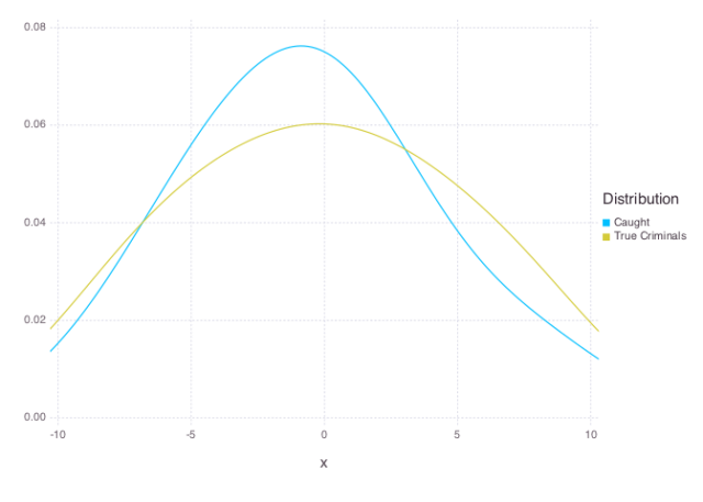
If you sample un-uniformly from a distribution, you don’t get the same distribution back.

I just finished an excellent book by Cathy O’Neil, called Weapons of Math Destruction. I would consider it an important book. Cathy explores, through dozens of contemporary, solid examples, the negative societal implications of naive implementation of statistical learning algorithms. In it, she makes concrete this exact scenario we are exploring here. She explores the software being developed and sold to police departments that predicts future crime based on past data.

In the real-life algorithms being implemented by police departments, as in our toy simulation, the data used to find criminals is not the data on crimes, but the data on crimes caught.

On day 52, our aspiring department uses, quite naturally, the data from day 51, which offers the most accurate predictions as to who will predict crime. The police are most definitely catching more criminals, but they are also biasing their statistics, and when those are the same statistics being used to catch the next batch of criminals, you have structural inequality.

This is what structural inequality looks like after 100 days of efficient policing:

Our police department has slowly, unwittingly, implemented the exact “efficient” strategy that the consultant originally proposed: sample from the mode, you will catch the most criminals. The police department is definitely working efficiently, if we narrow our definition of productivity to number of criminals caught, but they’ve created a whole new problem.

I’ll leave it to others to discuss the implications of the above distributions, the implications that structural inequality has for our society. But I hope this simulation has at least proved the statistical reality of the situation.

For those curious, here’s the code used for the simulations and graphs:

	using Distributions
	using Gadfly
	using StatsBase
	using KernelDensity
	using DataFrames
	function generate_population(n::Int, d::Sampleable)
	# Create population, with criminals distributed according to
	# the provided distribution (d)
	x = rand(n) * 20 – 10
	y = [pdf(d, i) > rand() ? 1 : 0 for i in x]
	collect(zip(x,y))
	end
	function catcher(population, estimate, unif::Bool)
	# If we are sampling uniformly, pick 1/10 of the population at random,
	# otherwise, use the previous estimated density function to sample.
	sampler = !unif ? x -> pdf(estimate, x) > rand() : x -> 1/10 > rand()
	# Stop people according to our sampling strategy. If we find
	# a 1, that indicates a criminal, and we catch them.
	stopped = [(x,y) for (x,y) in population if sampler(x)]
	caught = [x for (x,y) in stopped if y == 1]
	# Restimate a probability density based on those we caught
	estimate = InterpKDE(kde(caught))
	caught, estimate
	end
	function simulate(n::Int, K::Int, unif::Bool, d::Sampleable = Normal())
	# Generate our initial population
	pop = generate_population(n, d)
	# Run the catcher K times
	caught, _ = reduce((t, _) -> catcher(pop, t[2], unif), ([], d), 1:K)
	# Return the original criminals as well, to compare
	true_criminals = [x for (x,y) in pop if y == 1]
	caught, true_criminals
	end
	function create_df(caught, badguys)
	[DataFrame(x = caught, Distribution = "Caught");
	DataFrame(x = badguys, Distribution = "True Criminals")]
	end
	function resample(n::Int, K::Int, unif::Bool, d::Sampleable, geom, coords)
	caught, badguys = simulate(n, K, unif, d)
	df = create_df(caught, badguys)
	plot(df, x = "x", color="Distribution", geom, coords)
	end
	to_svg(plots) = [draw(SVG(n, 7inch, 5inch), p) for (n, p) in plots]
	d = Cauchy(0, 10)
	geom = Geom.density(bandwidth = 3)
	coords = Coord.cartesian(xmin=-10, xmax=10)
	to_svg([("day-one.svg", plot(x = simulate(1000000, 1, true, d)[2], geom, coords)),
	("uniformly-50.svg", resample(100000, 50, true, d, geom, coords)),
	("efficient-one.svg", resample(100000, 1, false, d, geom, coords)),
	("efficient-100.svg", resample(100000, 100, false, d, geom, coords))])

view raw

racists.jl

hosted with ❤ by GitHub